Data Visualization Applications: Slope Charts

This article is rated as:

Slope charts are an extension of line charts ideal for presenting changes over time. While line charts are effective at illustrating change over multiple time periods, slope charts excel at illustrating changes between two distinct time periods.

The benefits of opting for slope charts include:

•  Clarity in comparisons: Slope charts allow for easy comparisons between two points in time.

• Simplicity: By focusing on fewer data points (i.e., two time periods), slope charts simplify complex data. This makes slope charts more accessible to colleagues and clients.

• Identification of trends: Their simplicity allows for easy identification of trends and patterns, effectively illustrating increases, decreases, or stability between time periods.

• Enhanced storytelling: Slope charts clearly provide a visual narrative of change over time, making it easier to communicate key insights from the data.

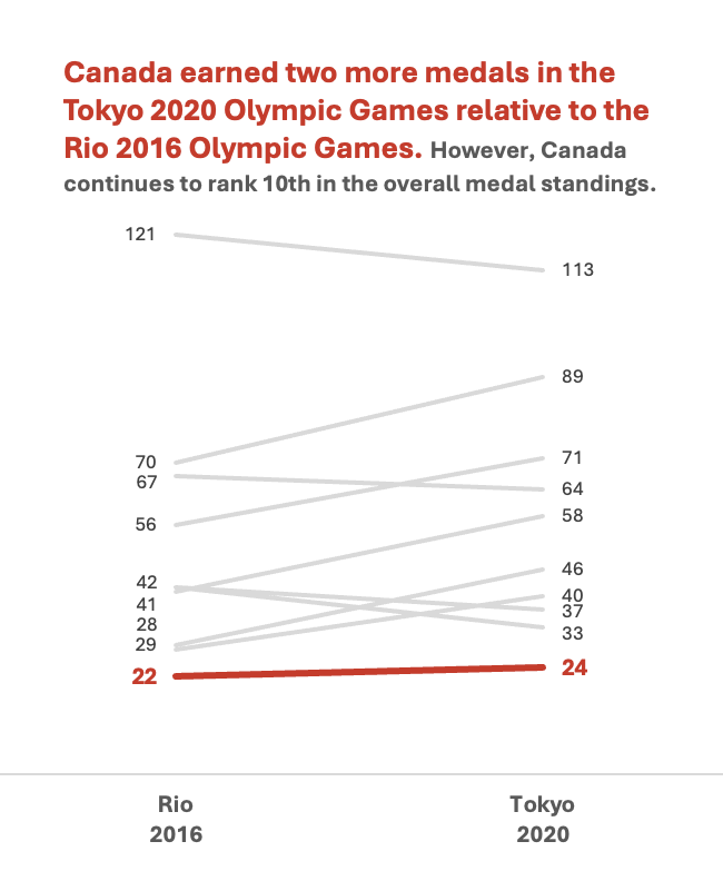
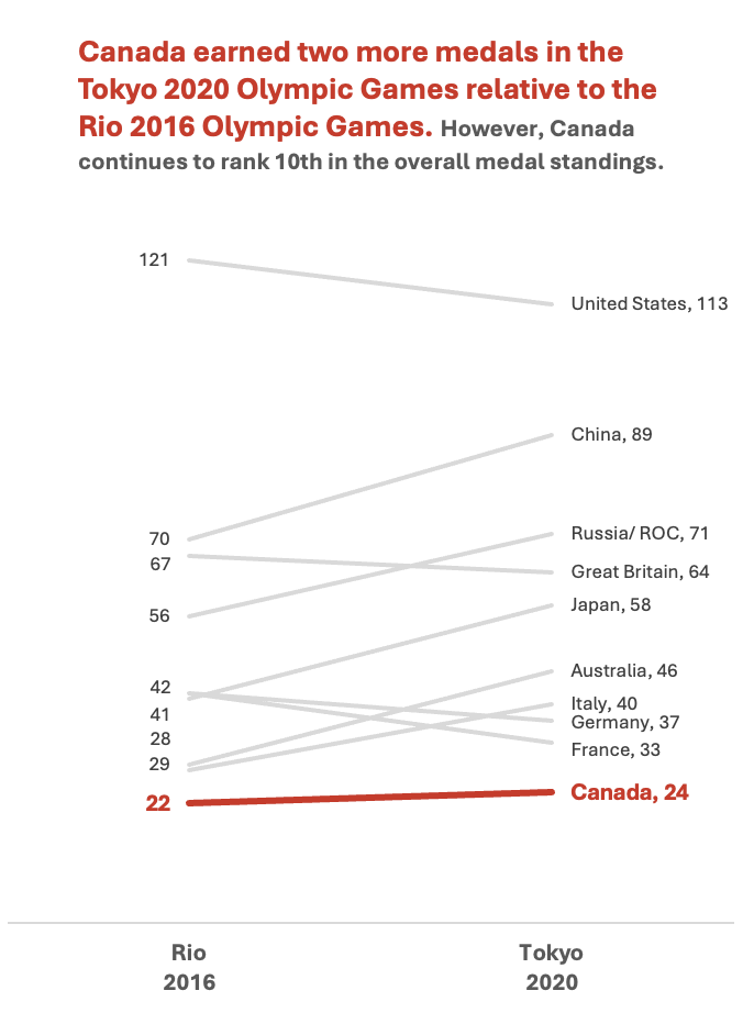
The Paris 2024 Olympic Games inspired us to reflect on the overall medal counts for the Top 10 countries from the previous two summer Olympic Games. We will use a slope chart to highlight changes between the Rio 2016 and Tokyo 2020 Olympic Games, with an emphasis on Canada (a perfect example of selection bias – see our articles on sampling bias and bias versus confounding to help avoid bias in your own analyses).

Check out the following Eval Academy resources to assist in preparing data for effective data visualization:

• The Data Cleaning Toolbox

• Let Excel do the Math: Easy tricks to clean and analyze data in Excel

• How to combine data from multiple sources for cleaning and analysis

• A Beginner’s Guide to PivotTables

Data Preparation

This article assumes that data are already prepared. That said, data should be structured in a clean and organized table like the example below.

Note: This table has prepared the Rio 2016 and Tokyo 2020 data labels such that the year number will be presented below the hosting city. This can be accomplished by using Alt+Enter at the end of the city name to move to the next line within the same cell.

Initial Chart Selection

1. Highlight the data to be included in the line chart.

2. Navigate to Insert along the top ribbon of Excel.

3. Within Insert go to Charts > 2-D Line > Line (a basic Excel-formatted chart should appear).

Applying Data Visualization Best Practices

Following this single step will have produced a line chart. This initial line chart needs to be converted to a slope chart, and improved by following data visualization best practices. This will transform the default Excel chart into an engaging visual.

Flipping Row/ Column Data

This example illustrates a common occurrence within Excel. Excel charts will often attempt to plot column headings along the x-axis of the chart (i.e., the horizontal axis) and row headings along the y-axis (i.e., the vertical axis). However, there is no need to transpose the data table to accommodate Excel’s plotting conventions. Instead, we can use the following steps to flip row/ column data within the chart.

1. Left-click within the slope chart.

2. Navigate to the Chart Design tab along the top ribbon of Excel.

3. Click Switch Row/ Column.

*Alternatively, you can right-click on the chart and go through Select Data… > Switch Row/ Column > OK. This menu also provides additional options for editing the data.

Lock Y-Axis Bounds

1. Right-click on the y-axis (i.e., the vertical axis).

2. Select Format Axis…

3. Under Axis Options > Bounds lock the Minimum to 0 and the Maximum to 150*

*This is not mandatory, but it can prove beneficial to lock the Bounds of a given axis. The Auto bounds will adjust with new data. However, sometimes the Bounds will become skewed as Excel tries to fit the data. That is, the Minimum Bound may exceed zero and potentially interfere with the accurate interpretation of the data.

Improve the Appearance

Remove the Legend

1. Left-click on the legend below the slope chart.

2. Hit Delete to remove the legend (we will improve upon this later). 

Line Thickness

1. Left-click on the Canada line within the slope chart (Canada is ranked 10th so this will be the bottom line).

2. Right-click the highlighted line and Format Data Series.

   • This menu can also be accessed using the Ctrl + 1 keyboard shortcut.

3. Under Series Options > Line adjust the Width of the line to 3 pt.

4. Complete the same process for the remaining nine (9) lines. However, we are going to mute these lines relative to the Canada line. Thus, we may opt for a slightly smaller line thickness (e.g., 2 pt).

Remove Clutter

1. Delete the y-axis labels by left-clicking on the y-axis and hitting Delete.

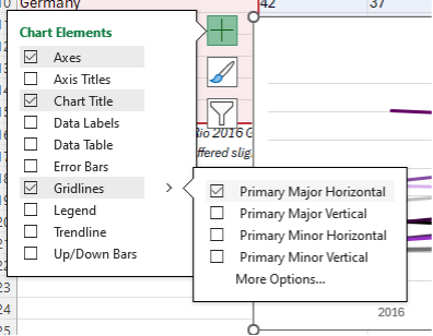
2. Delete the horizontal gridlines by left-clicking on the gridlines and hitting Delete.

   • Alternatively, you can navigate through the Chart Elements menu (the + like option when hovering over the chart) and toggle off Primary Major Horizontal gridlines.

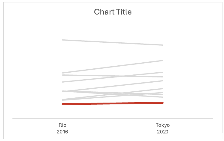
Highlight Key Data Points (& Mute Other Data Points)

In this example, we want to highlight Canada relative to the other Top 10 countries. Therefore, we want to make the Canadian data pop relative to the other countries. Line thickness helps (completed above), but colour will further highlight the Canadian data.

1. Right-click on the Canada line and change the Outline colour to red.

2. Repeat this process for each line, but change the remaining country colours to grey.

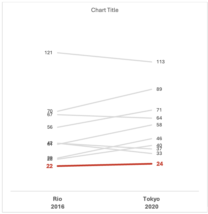
Insert Data Labels

1. Navigate to Chart Elements and toggle on Data Labels.

2. Right-click on a data label and select Format Data Labels…

3. For the Rio 2016 data labels, select the Left label position.

4. For the Tokyo 2020 data labels, select the Right label position.

5. Repeat this process for each data label.

Resize the Chart

The overlap in medal counts can clutter the chart. To help distinguish between different countries, the chart can be resized to better differentiate between each country's respective line.

1. Left-click on the chart and navigate to the Format tab at the top of the spreadsheet.

2. Resize the Shape Height to add some separation between lines.

Adjust Fonts

We want to further distinguish Canada from the other Top 10 countries. This can be accomplished with font size and colour.

1. Left-click on the chart to highlight the entire slope chart.

2. In the Home tab, select your Font of choice.

   • Sans serif fonts are best for charts. Ideally, chart fonts will match the rest of a report/ presentation to ensure consistency. However, if a report uses a serif font, you may opt to use a sans serif font within your charts for improved readability.

3. Adjust the Font Size to 9 pt.

   • 9 pt is our recommended minimum font size for charts.

4. Left-click on the Canada data labels and change the Font Size to 11 pt and Bold the font.

5. Also adjust the x-axis labels to 11 pt and Bold the font.

6. Change all Font Color to Black.

7. Left-click on the Canada data labels and change the Font Color to red.

Improve the Chart Title

The column heading will automatically default as the chart title. This will inevitably be uninformative. Therefore, update the chart title with something that is both descriptive and informative. 

1. Left-click on the Chart Title.

2. Type in your improved title and hit Enter.

   • The chart title may be edited within the function bar at the top of your spreadsheet.

   • You may also opt to right-click on the chart title and Edit Text to improve the chart title.

   • You can enter a subtitle by using Alt + Enter to move down a line.

3. Emphasize the chart title by increasing the main title to 14 pt font.

   • A subtitle, if you have one, can be de-emphasized using a slightly smaller 12 pt font.

   • When drafting the title within the line chart, you will have to highlight the specific section of text for which you wish to apply changes. Otherwise, all changes to the font will apply to the whole title.

4. Use your primary colour to further emphasize the main point within the chart title.

Manually Adjust Data Labels

Occasionally data labels will overlap partially or completely. This makes reading the chart difficult, but this can be improved with some manual tweaks to the chart.

1. Left-click on the overlapping labels and drag the higher value up or lower value down to provide some spacing.

   • This may take some patience to best align the data labels.

Adding in Descriptive Labels

Currently, the chart highlights Canada, which can only be identified via the chart title. However, all other lines are indistinguishable. We can improve this by adding in the country labels for each line.

1. Right-click on each of the right-most data labels individually.

2. Select Format Data Labels…

3. Under Label Options toggle on the Series Name

*Sometimes these additional labels will be too long and clutter the chart excessively. In this instance, United States of America, People’s Republic of China, and Russian Federation/ ROC were shortened to United States, China, and Russia/ ROC, respectively.

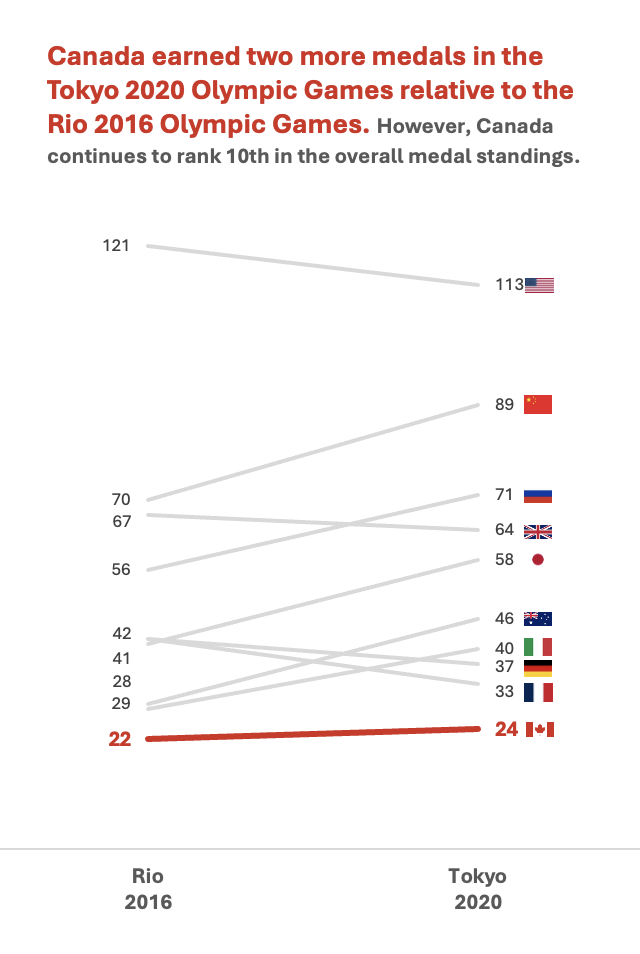
An Alternative to Descriptive Labels

To add some additional flare to your visuals, you may consider using images or icons to differentiate between data points. These data reflect medal counts by country, so the use of flags could be used to differentiate between lines within the chart. However, this approach should be used sparingly as not all charts lend well to the addition of images and some images may detract from the overall interpretation of the chart.

Final Thoughts

Slope charts are effective charts for illustrating change over time, making it easy to compare different data points. Their ability to simplify complex data and highlight trends enhances data storytelling, which will make reporting more digestible and engaging.