
A Beginner’s Guide To PivotTables
December 2021
This article is rated as:


If you work with data in Excel, whether frequently or infrequently, learning the basics of PivotTables will improve your ability to quickly explore and analyze raw data. PivotTables can transform your raw data into meaningful insights and reports in minutes. And the best part: creating PivotTables does not require any prior knowledge of Excel’s built-in formulas. With a few clicks of the mouse, you can generate fast, accurate results.
With PivotTables you will be able to quickly:
Summarize data (e.g., averages, counts, sums)
Sort data (e.g., alphabetically, numerically)
Group data (e.g., dates by month)
Filter data (e.g., by department, by region)
PivotTables let you go from rows and columns of raw data to results in just a few clicks (see the table below). Creating meaningful data summaries is a breeze with PivotTables, and once you understand the basics, you will not have to go back to using manual formulas for most of your reporting needs. Just let PivotTables do all the work for you.

This article will walk you through the basics of working with PivotTables, using sample data from patient surveys conducted in medical clinics.
Preparing your data
Before jumping into working with PivotTables, we need to take care of some basic housekeeping. While there are several ways of entering data into an Excel spreadsheet, data should be entered in a tabular format such that:
The first row contains a clear header describing the data in the columns
Each column should only contain data of a single type (e.g., a Date column should only contain dates)
Each row should only contain data from a single time point (e.g., a program participant may answer a survey on two different dates, but each survey should be entered into its own row)

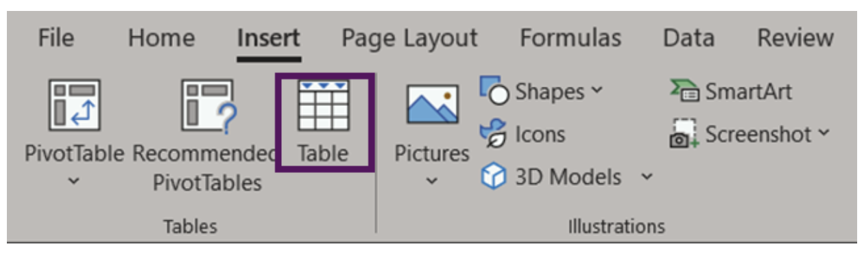
The data are now ready to be used in a PivotTable. It is possible to create a PivotTable using the as formatted above. However, if you were to enter new data to the spreadsheet, the PivotTable would not automatically update with the new data. Luckily, there is an easy fix for this: convert the data range into an Excel Table (Insert > Table OR Ctrl + T). An Excel Table organizes the data and makes it easy to sort, filter, and format.
The appearance of your Tables can be edited within the Table Design tab. Within this tab you can change appearance of your Table with preset Table Styles, or even opt to remove all formatting completely. You may also want to give your Table a name (located on the left of the Table Design tab). Naming the spreadsheet becomes important when you are working with many data Tables and PivotTables, as these names will allow for easy reference.

Inserting a PivotTable
With data organized into a Table, it is time to insert a PivotTable. There are a couple of options:
1. Insert > PivotTable
Click anywhere within your Table
Navigate to the Insert Tab (top left of Excel spreadsheet)
Select ‘PivotTable’ (or ‘Recommended PivotTables’)*
2. Table Design > Summarize with PivotTable
Click anywhere within your Table
Navigate to the Table Design tab (top right of Excel spreadsheet)
Select ‘Summarize with PivotTable’
*‘Recommended PivotTables’ will provide recommendations for summarizing your data in a PivotTable. This is a good option if you are unsure of how to summarize your data.
Both options will bring up the ‘PivotTable from table or range’ pop-up box. Within this box, you can select your Table or Range, if you have not done so already; the name of your Table would show here if you converted your data into a Table prior to inserting a PivotTable. You can also select where the PivotTable will be placed: (1) to a New Worksheet or (2) to an Existing Worksheet.

Note: ‘Add this data to the Data Model’ will allow you to perform more complex tasks on your PivotTable, including the ability to create your own formulae within a PivotTable or the ability to link two or more PivotTables together based on a common attribute. However, these are more advanced skills and are not covered in this article.
Getting familiar with PivotTables
Unless you used the ‘Recommended PivotTables’, your PivotTable will not look like much. You will be presented with an empty PivotTable located within the spreadsheet and a PivotTable Fields menu on the right-hand side of your workbook. We will start with the PivotTable Fields menu to really get started working with PivotTables.

There are many ways to organize your data within a PivotTable. Using the data presented above, let’s look at the ‘Rating of Care Received’ first.
Summary of ‘Rating of Care Received’
Within the PivotTable Fields menu toggle on ‘Rating of Care Received’ (or click and drag)
‘Rating of Care Received’ will be added to the Rows field
Navigate back to ‘Rating of Care Received, and click and drag the option down to the Values field

Note that as you drag and drop data into their respective field, the table in the spreadsheet will update. This provides you within instantaneous feedback. If you drop data into the wrong field, simply click and drag the data outside of the box and it will be removed from the PivotTable.
We now have a basic summary of the Counts of survey participants based on their response to the ‘Rating of Care Received’ question. However, you’ll notice that the Row Labels are ordered alphabetically. PivotTables will automatically organize text date alphabetically; numbers will be ordered numerically, and dates will be ordered chronologically. This is likely not the order that you’d prefer the data to be organized in. To reorder the Row Labels, you can click on a label (e.g., Very good) and drag it to the desired location (e.g., below Excellent).

The data are currently summarized at the aggregate level. That is, all survey responses, regardless of Date, Clinic, Gender, or Age Range are summarized in the PivotTable. But you would probably like to summarize the data at a more granular level.
‘Rating of Care Received’ by Date
Click and drag the Date data into the Columns field

Immediately, you will notice that when you drag the Date data into the Columns field, the Columns field populates with Years, Quarters, and Date. This will occur automatically for dates (if the data are formatted properly as dates). But you may not want all these additional levels added to the PivotTable. For undesired labels, simply click and drag to remove. In this example, we want only Years and will remove the Quarters and Date information.

Note: Dates can be grouped by Seconds, Minutes, Hours, Days, Months, Quarters, and Years. By right-clicking on the Date labels in the PivotTable you will get a menu with the option ‘Group’. This will open a menu where you can select the grouping level you desire. If you do not want the data grouped, right-click on the Date labels in the PivotTable and click the ‘Ungroup’ option from the menu.
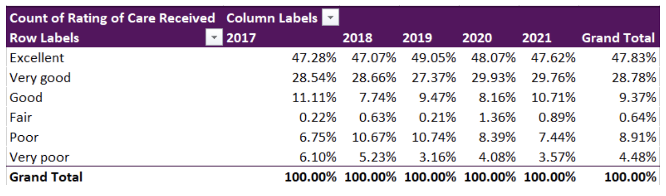
We now have the Counts of each response from 2017 to 2021. This may be good enough, but having the percent response rate will allow for better comparisons between years.
Counts to Percent of Column Total
Within the PivotTable Fields menu, click the arrow of Count of Rating of Care Received within the Values field
Select Value Field Settings from the pop-up menu
Select Show Value As within the Value Field Settings menu
‘Show value as’ the % of Column Total

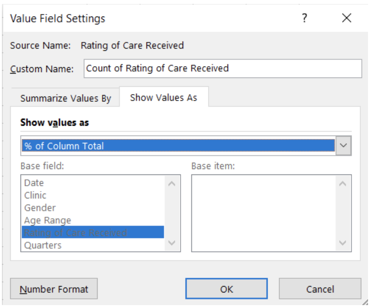
The ‘Rating of Care Received’ data will now be summarized as the percent of the column total (i.e., summarized by Year).
Again, these results may be sufficient for your reporting needs. However, you may be asked to break the data down by a specific group. This can be accomplished with Filters and Slicers. A Filter is a built-in drop-down menu within the PivotTable, while a Slicer is a separate filter menu that moves independently of the PivotTable. Both are used to filter data based on one or more variables. However, a Slicer has the added benefit of being able to link to multiple PivotTables. Selecting a filter option within a Slicer can apply the filter across multiple, linked PivotTables at the same time.
Adding a Clinic Filter
Drag the Clinic data into the Filters field

Adding a Clinic Slicer
Navigate to the PivotTable Analyze tab at the top right of the workbook
Select ‘Insert Slicer’

You now can actively filter your data using either the Filter or Slicer option. This is beneficial when you do not need to present all clinics’ data at the same time. It also offers interactivity within the spreadsheet, where different clinic results can be prepared with a few clicks.
Adding multiple variables to PivotTable fields
With the previous example, we only entered a single variable per PivotTable field (Filters, Rows, Columns, and Values). However, you can add as few, or many, variables as needed in each field. Note that with Columns, Rows, and Values the data will become nested and the PivotTable can become expansive quickly. For example, by pulling the Clinic data out of Filters and moving it into the Rows field, we can get a summary by clinic within the same PivotTable.

Because PivotTables update quickly as you drag and drop variables into the different fields, I recommend experimenting with your PivotTables in the beginning. With experience and experimentation, you will get a better feel for how PivotTables should be organized to best summarize your data. PivotTables are powerful tools, and this quick walkthrough only scratches the surface of what PivotTables can do.
Up your PivotTable game
Design
If desired, you can accept the default PivotTable format. But, if you’re anything like me, you will want to change the PivotTable design as soon as possible. Luckily, this is simple. When clicked within your PivotTable, a Design tab will appear at the top right of the Excel workbook (next to PivotTable Analyze). Within this tab, you have the option of changing the style and colours of your PivotTable. You also have the option to insert headers, banded rows, and banded columns. Further, you have options to include or exclude data summaries (e.g., row or column totals).
The Design tab will drastically improve the look of your PivotTables. Match to your company or clients’ colours or select a design that distinguishes between different datasets. Or, if you prefer, remove all design formatting for a less distracting appearance.

Grouping non-date data
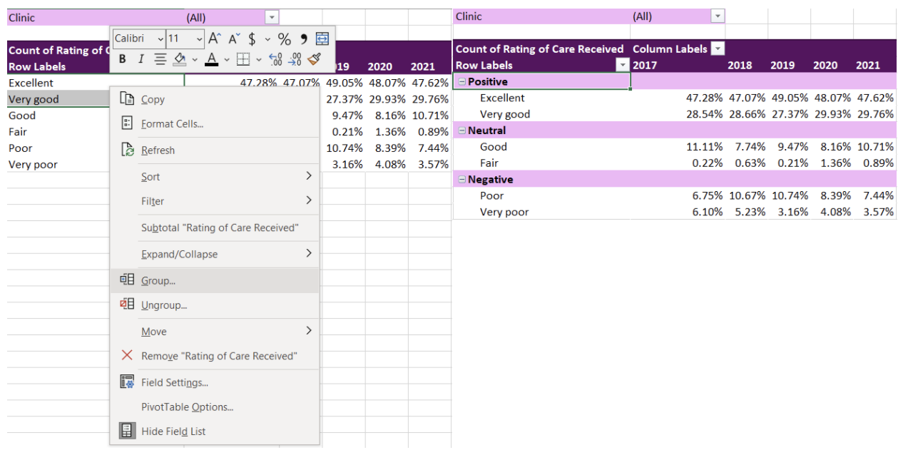
I briefly discussed how dates are grouped within PivotTables. Just as with dates, other variables can be grouped too. For example, with the ‘Rating of Care Received’ row labels, you may want to group the responses into fewer categories (e.g., Positive responses = Excellent, Very good; Neutral responses = Good, Fair; Negative responses = Poor, Very poor). To group the labels, highlight the labels you wanted grouped (e.g., Positive responses = Excellent, Very good) and right click. Navigate to the ‘Group’ option within the menu. This will group these labels under ‘Group 1’, which can be changed to any group title you want by simply writing within the group label cell.
Using Slicers to connect two or more PivotTables
Like I mentioned previously, it is possible to link multiple tables to the same Slicer. With the Slicer already created in the previous example, adding an additional linked PivotTable is easy. For this example, I copied the original PivotTable creating two identical PivotTables. For simplicity, I filtered the Column Labels to present only 2020 in the first PivotTable and 2021 in the second PivotTable.
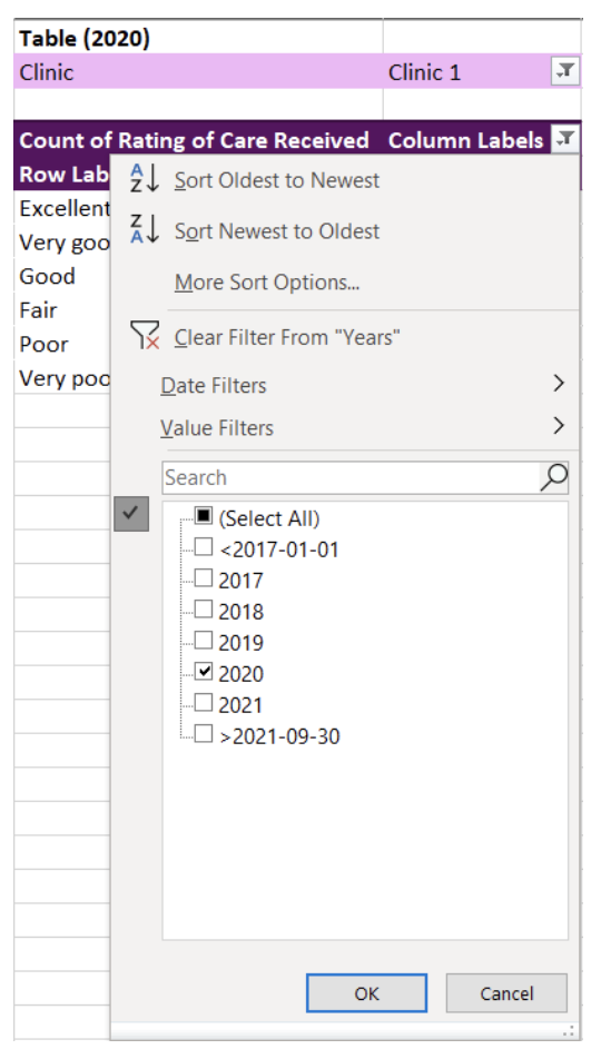
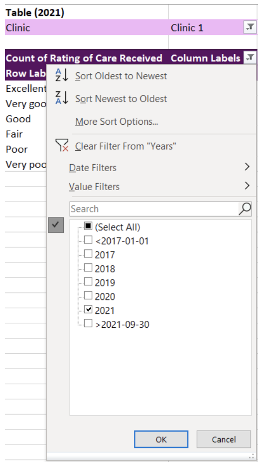
To link a Slicer to the two PivotTables, right click a Slicer that you have already created. From our example, this is the Clinic Slicer. From the menu, navigate and select Report Connections to bring up all potential connections for the Slicer. The list of Report Connections will list the different PivotTables for which it can connect. Simply toggle on all PivotTables you want to connect to the Slicer.


You will now have two PivotTables that can be filtered simultaneously with the click of button. Select any option within the Slicer and both PivotTables will update. You can use this approach to link several PivotTables and can be useful for designing interactive dashboards within Excel.
You should now have the fundamentals to begin working with PivotTables. With no background knowledge of Excel formulas required, PivotTables offer a fast, accurate, and intuitive alternative to organize and analyze your data.
The ease and flexibility of PivotTables encourages experimentation. And the best method for mastering PivotTables is to jump in and experiment with your data. Soon you’ll be able to tie in all these fundamentals to generate insights with ease.